Simulation of a Rotary Inverted Pendulum in Matlab-Simulink.
The Rotary Inverted Pendulum (RIP) problem is a popular control theory project, and it exemplifies a classic challenge in dynamic systems and control engineering. This system, also known as the Furuta Pendulum, involves a pendulum attached to the end of a rotating arm, where the primary goal is to control the arm’s rotation to keep the pendulum balanced upright. It presents a real-time test of stabilization techniques, as it is inherently unstable and requires continuous feedback and adjustments to maintain equilibrium. The problem is widely used to demonstrate principles of linear and nonlinear control theory, including PID control and state space representation techniques.
Developing the dynamic model
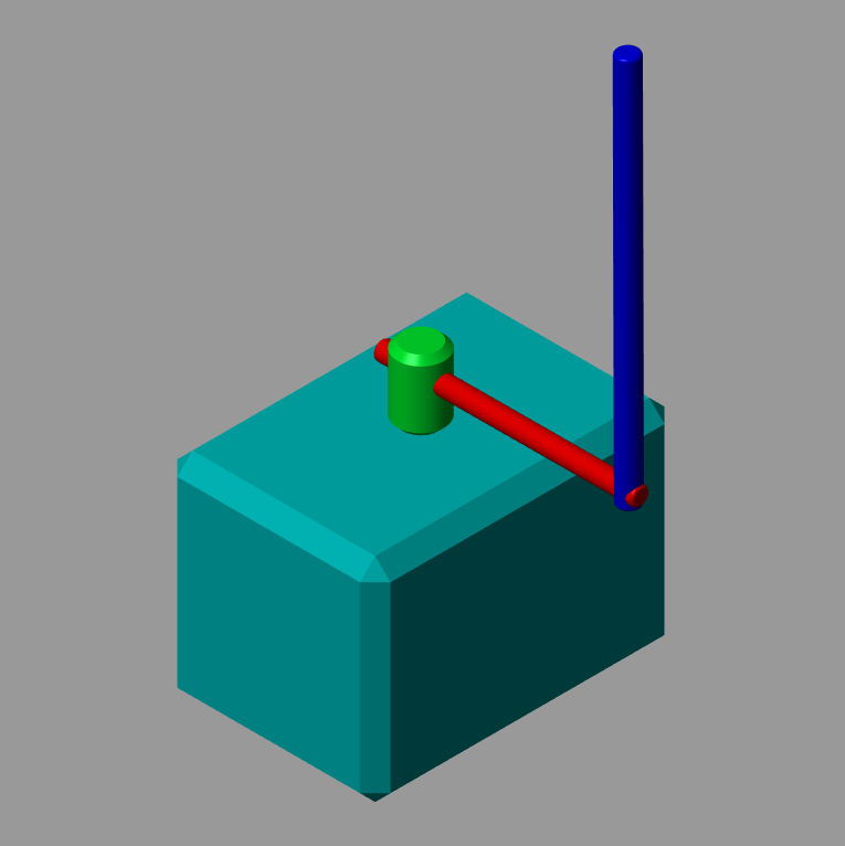
The design of this system is quite simple, and it consists of only two main parts and connecting components. It was modeled first in SolidWorks and then imported into Simulink using the Simscape Multibody toolbox. The various dimensions and parameters of the modeled system can either be taken note of at this point to be fed into the controller or conversely, they can be directly referenced from the XML file generated by the import. I have found the former to be simpler and easy to implement while not a very scalable method, but should suffice for this example.
Modeling the system
First step for designing any controller is writing the equations of motion that define the system.
We write the equations of motion as:
\[(mL_r^2 + \frac{1}{4}mL_p^2 - \frac{1}{4}mL_p^2\ cos(\alpha)^2 + J_r)\ddot \theta - \frac{1}{2}mL_pL_r\ cos(\alpha)\ddot \alpha + \frac{1}{2}mL_pL_r\ sin(\alpha)\dot \alpha^2 = \tau - D_r\dot \theta\] \[-\frac{1}{2}mL_pL_r\ cos(\alpha)\ddot \theta - (J_p + \frac{1}{4}mL_p^2)\ddot \alpha - \frac{1}{4}mL_p^2\ sin(\alpha)\cos(\alpha)\dot\theta^2 - \frac{1}{2}mL_pg\ sin(\alpha) = D_p\dot\alpha\]Here, $\theta$ is the angle of the pendulum from the vertical axis, $\alpha$ is the angle of the arm from the horizontal axis, $L_r$ is the length of the arm, $L_p$ is the length of the pendulum, $m$ is the mass of the pendulum, $r$ is the distance of the pivot point from the center of mass of the pendulum, $J_p$ is the moment of inertia of the pendulum about its center of mass and $J_r$ is the moment of inertia of the arm. Additionally, we have $D_p$ and $D_r$ ,which are the damping coefficients of the pendulum and arm respectively.
Linearization
Next, we linearize the system of equations. In our case, we want the pendulum to stay upright, so that would mean $\theta = \pi$ and additionally, we want $\alpha = 0$. Based on these conditions the linearized equations of motion would be:
\[(mL_r^2 + J_r)\ddot \theta - \frac{1}{2}mL_pL_r\ddot \alpha = \tau - D_r\dot\theta\] \[-\frac{1}{2}mL_pL_r\ddot\theta +(J_p + \frac{1}{4}mL_p^2)\ddot\alpha - \frac{1}{2}mL_pg\alpha= D_p\dot\alpha\]Designing the PID controller
PID control is a very straightforward approach to the problem, which works by adjusting the control output based on the proportional, integral and derivative terms of the error signal. It is a good way to quickly get the project off the ground and test basic functionality, and will provide sufficiently good results with relatively less effort. The most tedious part of this method is tuning the controller gains, and there are several methods to do this, including Ziegler-Nichols and Cohen-Coon.
Because we have two control inputs, $\theta$ and $\alpha$, we need two PID controllers, $c_{\theta}$ and $c_{\alpha}$. The transfer functions for these two controllers can be derived from the linearized equations.
The general form of the transfer function for these controllers would be:
\[C(s) = K_p + \frac{K_i}{s} + K_ds\]Once we have good enough values for the controller gains, we now have a controller that can maintain the system at equilibrium.
Designing the state space controller
A PID controller is good enough to begin with, but as we notice, it cannot handle large errors or disturbances, and the system immediately goes awry.
This is mainly due to two factors:
-
PID controllers are inherently linear. They are designed to perform well around a tiny operating range, in a very small region around the equilibrium point at which we have linearized the system. An RIP exhibits highly nonlinear dynamics, especially as the error becomes large, and the dynamics can no longer be approximated as linear, and this throws the controller into discord.
-
PID controllers can only be used for Single Input Single Output (SISO) systems. In our case, we have chosen only one state to monitor, and that is the angle of the pendulum, $\theta$. To better control the system, we must also ensure the angle of the arm, $\alpha$ be maintained.
A state space controller solves these issues. It can handle Multiple Input Multiple Output (MIMO) systems and it has a wider range of operating conditions around the equilibrium point.
Designing a state space controller requires some more steps after linearization.
First we write the state equations
\[\dot X = Ax+Bu\] \[Y = Cx + Du\] \[X = \begin{bmatrix}\theta\\\alpha\\\dot\theta\\\dot\alpha \end{bmatrix}\] \[Y = \begin{bmatrix} \theta \\ \alpha \end{bmatrix}\]Now we find the matrices $A$, $B$, $C$ and $D$. This is done by first finding $\ddot \theta$ and $\ddot \alpha$ in terms of the physical parameters of the system and then converting the linearized equations into the state space formulation.
\[A = \frac{1}{J_T}\begin{bmatrix} 0&0&1&0 \\0&0&0&1 \\0 & \frac{1}{4}m^2L_p^2L_rg & -(J_p+\frac{1}{4}mL_p^2)D_r & -\frac{1}{2}mL_pL_rD_p \\0 &\frac{1}{2}mL_pg(J_r +mL_r^2) & \frac{1}{2}mL_pL_rD_r & (J_r + m_pL_r^2)D_p \end{bmatrix}\] \[B = \frac{1}{J_pmL_r^2+J_rJ_p+\frac{1}{4}J_rmL_p^2} \begin{bmatrix} 0\\0\\J_p + \frac{1}{4}mL_p^2\\\frac{1}{4}mL_pL_r \end{bmatrix}\] \[C = \begin{bmatrix} 1&0&0&0 \\ 0&1&0&0 \end{bmatrix}\] \[D = \begin{bmatrix} 0\\0\end{bmatrix}\]The final step once we have these matrices is to design the observer based state-feedback controller. Determining the state feedback matrix $K_c$ is the first stage of this process, and for that we determine the desired closed-loop pole locations, with the help of the place() method in MATLAB. The second stage is placing the observer poles, $L_o$, at least five times as far away from the origin as $K_c$. This can also be done using the place() function.
Finally, we plug all of the above determined values into the State Space Controller block in Simulink to arrive at our desired controller.
With this controller, we see the performance of the RIP to have improved, even with large disturbances.
Final thoughts
State space controllers represent a significant step in control systems, yet they are not the pinnacle of error management and equilibrium maintenance. Advanced methods, including optimization-based strategies like the Linear Quadratic Regulator (LQR), enhance system performance through the minimization of a predetermined cost function. Beyond LQR, approaches like Model Predictive Control (MPC) offer further sophistication by anticipating future states and making adjustments accordingly. Additionally, adaptive control methods adjust to system changes in real-time, ensuring optimal performance under varying conditions. These methodologies extend the capabilities of traditional controllers, offering improved precision and adaptability.