Nesterov’s Accelerated Gradient Descent Method

Optimization is a branch of mathematics focused on finding the optimal solution to a problem. The ‘problem’ is represented by a multivariate function, known as the objective function, with the variables being parameters that we wish to optimize. Optimization is used extensively in computer science, particularly in fields like machine learning for fine-tuning hyperparameters of neural networks, and in robotics for determining the most optimal path for a robot, considering various path-related costs.

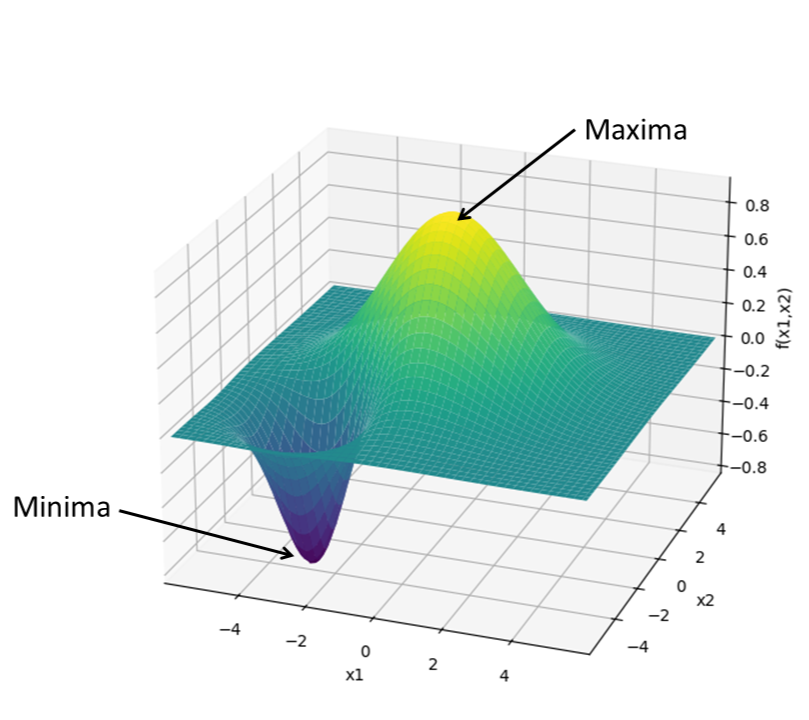
One way to visualize an optimization problem is by plotting the objective function against its variables. For instance, consider this 2-dimensional function:

\[f(x_1, x_2) = e^{\left(\frac{x_1^2}{8} - \frac{x_2^2}{8}\right)} - e^{\left(-\frac{(x_1 + 3)^2}{2} - \frac{(x_2 + 3)^2}{2}\right)}\]

The task now, is to find the values of $x_1$ and $x_2$ for which the value of the function is either the highest, known as the maxima, or more commonly the lowest, known as the minima, based on what type of optimization problem it is.

Gradient descent

One of the most widely used optimization techniques is gradient descent (GD), which finds the minimal solution by iteratively moving towards the steepest descent direction of the objective function, which is the negative of the gradient at that point. The formula for gradient descent is:

\[x_{k+1} = x_k - \alpha \nabla f(x_k)\]

Where $\nabla f(x_k)$ is the gradient of the function at the current value $x_k$ of the input $x$. The way the update rule is set up moves each iteration closer to where the gradient, $\nabla f(x)$, would be zero, and this is usually where either the maxima or the minima lies.

Vanilla GD is generally reliable, but it faces issues with saddle points, which are points with zero gradients, but are neither minima nor maxima. GD may also encounter large plateaus, which are often mistaken for saddle points, and can slow down convergence significantly leading to the algorithm getting stuck.

Nesterov’s and other momentum based methods

Momentum-based techniques enhances GD methods by adding a momentum term to the update rule. The momentum term helps accelerate convergence, especially in the presence of large, flat regions and steep, deep valleys. The update rule for momentum-based gradient descent is:

\[v_{k+1} = \beta v_k + \alpha \nabla f(x_k)\] \[x_{k+1} = x_k - v_{k+1}\]

Here, $v_k$ is the velocity vector, and $\beta$ is the momentum coefficient, typically between 0 and 1. The momentum term $\beta v_k $ allows the algorithm to build speed in directions with persisting gradients, i.e., if the gradient value is the same for consecutive iterations, it would place higher trust in that gradient, and thus, would increase the speed, helping it navigate large plateaus and accelerate convergence.

Nesterov’s Accelerated Gradient (NAG) further refines this approach by making a slight adjustment. Instead of calculating the gradient at the current position, NAG computes it at a lookahead position, giving a more informed update:

\[v_{k+1} = \beta v_k + \alpha \nabla f(x_k - \beta v_k)\] \[x_{k+1} = x_k - v_{k+1}\]

This lookahead step allows NAG to anticipate the future trajectory and make more accurate updates, resulting in faster convergence and better performance.

For a detailed look at how the math behind NAG works, please check out this paper detailing the method as well as the proof of the improved convergence rate.

Implementation

Let’s now write a simple implementation to visualize the superiority of NAG over GD.

Let’s define the objective function, a rift function, similar to what you would encounter in tuning the parameters of a neural network based on the error term of the sigmoid neuron. The function can be defined as:

\[f(x_1,x_2) = e^{-(\frac{x_1^2}{20} + \frac{x_2^2}{5})}\]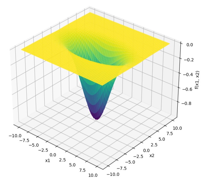

From the definition, it is visible that $f(x_1, x_2)$ attains its minima when the exponential term is maximized, since the exponential function $e^{-x}$ decreases as $x$ increases. The exponential term $-(\frac{x_1^2}{20} + \frac{x_2^2}{5})$, in turn, is maximized when $(\frac{x_1^2}{20} + \frac{x_2^2}{5})$ is minimized, and the minimum value of $(\frac{x_1^2}{20} + \frac{x_2^2}{5})$ is $0$, which occurs at $x_1 = 0$ and $x_2 = 0$.

With this knowledge, let’s proceed to see how close and how quickly both methods converge to the value $(0,0)$.

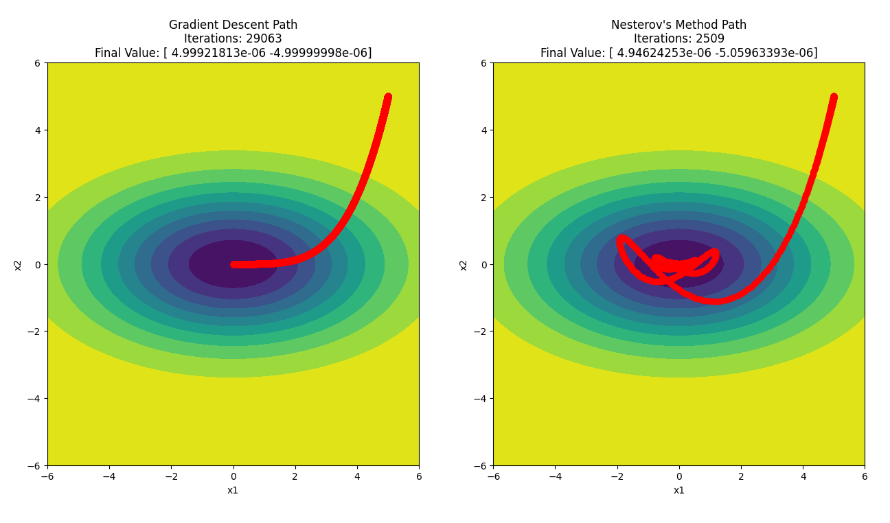
By running the two algorithms side-by-side, we notice a few things. Firstly, NAG converges faster than GD, as expected, by a factor of approximately 10 iterations, and both methods converge within similar distance from $(0,0)$, both in the order of $10^{-6}$. Secondly, the path taken by NAG to reach the minima isn’t straightforward like GD’s. There are a lot of turns in the path, almost like the algorithm makes it go one way, rethinks, and makes it take a “u-turn”.

The explanation for this is that NAG calculates the gradient at a future point, and not at the current point, unlike regular momentum-based methods, which allows NAG to adjust its course more frequently, leading to the observed “u-turns” and sudden changes in direction. These adjustments are a result of the algorithm constantly reassessing the path based on both the current gradient and the expected future gradient. This is why NAG can converge faster and more efficiently navigate complex terrains in the optimization landscape compared to the more straightforward but potentially less adaptive path of simple momentum-based and even GD methods.

The intensity of these “u-turns” can be minimized by carefully tuning the momentum parameter. If the momentum is set too high, the algorithm may overshoot and make larger, more frequent adjustments, but will expedite the convergence. Conversely, a lower momentum value can help smooth out the path by reducing the abrupt changes in direction, leading to a more stable yet slower convergence. Proper tuning would ensure that NAG maintains its efficiency advantage while mitigating excessive oscillations.

Conclusion

Nesterov’s method addresses the main issue with vanilla GD, which was slow convergence, and ensures that large plateus and deep valleys are traversed quicker. However, it shares some limitations with other momentum-based methods, including overshooting and oscillations in certain scenarios, as well as inherent issues with gradient descent methods, such as the saddle point problem.

To compensate for these issues, more advanced optimization algorithms have emerged, offering superior performance. Notable examples include RMSprop and ADAM, which adaptively adjust learning rates to enhance convergence speed and stability.

For a visual comparison of various optimization techniques, refer to the video below. It illustrates how different methods, represented by colored balls, approach finding the minima in a given topology. Specifically, the cyan ball represents vanilla GD, the magenta ball is a momentum-based method, the white ball Adagrad, the green ball RMSprop, and the blue ball representing ADAM. This video demonstrates the efficiency and robustness of modern algorithms like RMSprop and ADAM compared to traditional approaches.

For the full codebase, follow the link to the github repo