State Estimation of Autonomous Vehicles using Extended Kalman Filter

State estimation is an important technique used in fields such as robotics and aerospace, where true system states are often obscured or indirectly observed through noisy sensors. Techniques like Extended Kalman Filter (EKF) are employed to infer these hidden states by making use of mathematical models and measurements.

EKF helps to combine predictions about the system’s behavior, which are based on its dynamics rooted in theory, with actual noisy sensor readings, both of which can be inaccurate. By continually updating its estimates with new sensor data, EKF adjusts for uncertainties and errors, refining its predictions over time. This process allows the system to maintain accurate and reliable information about its state, which is essential for tasks like navigation, control, and decision-making, ensuring that the system operates effectively even in the presence of unpredictable factors.

Problem statement

Let’s now imagine that we have an autonomous vehicle, represented by the Dubins Car Model. This can be defined as a system with a state vector given by

\[x = \begin{bmatrix}p_x \\p_y\\ \theta \\ v \\ \phi \end{bmatrix}\]

and a transition vector given by

\[\dot x= f(x,u) =\begin{bmatrix} \dot p_x \\ \dot p_y\\ \dot \theta \\ \dot v\\ \dot \phi\end{bmatrix} = \begin{bmatrix} v\ cos(\theta) \\v\ sin(\theta)\\\frac{v}{L}tan(\phi)\\a\\ \psi\end{bmatrix}.\]

We want to control the car’s motion in its configuration space with the help of the control vector given by

\[u = \begin{bmatrix}a \\ \psi \end{bmatrix}.\]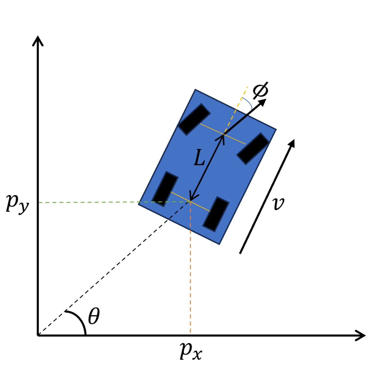

Here, $(p_x,p_y)$ is the position of the robot in the start frame, the heading, $\theta$, is the angle it makes with the horizontal axis of the start frame, $v$ and $a$ are the velocity and acceleration respectively of the robot in the direction of movement. $\phi$ is the steering angle, which is the angle the wheels make with the rest of the vehicle, and $L$ is the turn radius, which is also the distance between the front and rear axles of the robot-vehicle.

Our problem is that we do not have a direct reading of its state space. Instead we have a GPS sensor that can calculate the car’s forward velocity $v$, the heading rate $\dot \theta$, and the global coordinates $(g_x, g_y)$. The GPS sensor is located at point $(g_x^{ref}, g_y^{ref})$ in the robot’s start frame. Thus, the measurement vector can we written as

\[z = \begin{bmatrix}v\\\dot\theta\\g_x\\g_y \end{bmatrix}\]

Inaccuracies in the system

On testing, however, we find out that there are errors in the dynamics model. This is to be expected, since Dubins Car is only a theoretical model of a real vehicle’s dynamics, and theory will only take you so far.

The results of testing gives us reason to believe that

1. Due to physical issues with the acceleration pedal, the set acceleration $a$ may have an error of standard deviation $\lvert a \rvert \cdot \sigma_a$.

2. There might be an error in the steering angle, $\phi$, causing the heading $\theta$ to deviate, especially at high speeds. This error has the standard deviation $\lvert v \rvert \cdot \sigma_\theta$.

3. The vehicle’s position slips occassionally, and the velocity error in the forward direction is estimated to have a standard deviation $\lvert v \rvert \cdot \sigma_{fwd}$ and the error in the sideways direction has an SD of $ \lvert v \rvert \cdot \ \sigma_{side}$.

We also discover during testing that there are noises in the GPS sensor’s observation

1. The magnitude of error in velocity increases with velocity, and the standard deviation is given by $\lvert v \rvert \cdot \sigma_v$.

2. Heading rate measurement has errors with SD $\sigma _{\dot \theta}$

3. Both $x$ and $y$ direction readings have errors with SD $\sigma_g$

Solving the Problem

Let’s now see how we can solve this problem with the help of an EKF.

In EKF, the process begins with a prediction step using a predefined mathematical model of the system dynamics, which estimates the state forward in time. This model is typically represented as a system of differential equations, which in our case is the Dubins Car Model.

Then, the update step adjusts this prediction based on new sensor measurements. The relationship between the measured values and the system states is defined by a measurement model, which like the system model, can be nonlinear and needs to be linearized in the context of EKF.

Both the system and measurement models are subject to uncertainties. EKF addresses this by assuming that both the process and measurement noises are Gaussian, which simplifies the computation of the Kalman gain—a factor that determines the weighting of the new measurement relative to the prediction.

Building the model

The first step is to gather and understand all the components that are required to make the process work smoothly.

First, our state vector, $x$, given in the problem, to be

\[x = \begin{bmatrix}p_x \\p_y\\ \theta \\ v \\ \phi \end{bmatrix}\]

Next our transition vector, $f$, also given

\[f(x) = \begin{bmatrix} v\ cos(\theta) \\v\ sin(\theta)\\\frac{v}{L}tan(\phi)\\a\\ \psi\end{bmatrix}\]

Our control vector, $u$,

\[u = \begin{bmatrix}a \\ \psi \end{bmatrix}\]

And finally our measurement function, $h(x)$ which is a mapping from the state space to the measurement space. We know the measurement vector is

\[z = \begin{bmatrix}v\\\dot\theta\\g_x\\g_y \end{bmatrix}\]

We are also told that the GPS sensor is at $(g_x^{ref}, g_y^{ref})$ on the robot, but we know that to transform a point from one frame to other, we have to rotate and translate it.

\[\begin{bmatrix}g_x\\g_y \end{bmatrix} = R(\theta)\begin{bmatrix} g_x^{ref} \\g_y^{ref}\end{bmatrix} +\begin{bmatrix} p_x\\p_y \end{bmatrix}\]

But

\[R(\theta) =\begin{bmatrix} cos(\theta) &-sin(\theta) \\sin(\theta)&cos(\theta)\end{bmatrix}\]

So, by further calculation we get :

\[\begin{bmatrix} g_x \\g_y\end{bmatrix} = \begin{bmatrix} cos(\theta) &-sin(\theta) \\sin(\theta)&cos(\theta)\end{bmatrix}\begin{bmatrix} g_x^{ref} \\g_y^{ref}\end{bmatrix}+ \begin{bmatrix} p_x\\p_y \end{bmatrix}\] \[= \begin{bmatrix} p_x + g_{x}^{ref}cos(\theta) - g_{y}^{ref}sin(\theta) \\p_y+g_{y}^{ref}cos(\theta) + g_{x}^{ref}sin(\theta)\end{bmatrix}\]

Therefore, by substituting it into the original $z$ vector we get

\[h(x) = \begin{bmatrix} v \\\frac{v}{L} tan(\phi)\\p_x + g_{x}^{ref}cos(\theta) - g_{y}^{ref}sin(\theta) \\p_y+g_{y}^{ref}cos(\theta) + g_{x}^{ref}sin(\theta)\end{bmatrix}\]

Linearizing the model

The next step is to linearize the given model. This is necessary because an EKF, like a standard Kalman Filter, can only predict the states of linear systems. The EKF extends this capability to non-linear models by approximating them as linear at each time step around the current estimate, thus allowing it to handle non-linear systems effectively.

To linearize the model, we find the Jacobians of the vectors we gathered before. To do that we need to find the partial derivatives

\[F_t = \frac{\partial f}{\partial x};\ g_t = \frac{\partial f}{\partial u};\ H_t = \frac{\partial h}{\partial x}\]

By calculating these, we get

\[F_t = \begin{bmatrix}0 & 0 & -v \sin(\theta) & \cos(\theta) & 0 \\ 0 & 0 & v \cos(\theta) & \sin(\theta) & 0 \\ 0 & 0 & 0 & \frac{\tan(\phi)}{L} & \frac{v \left(sec^2(\phi) \right)}{L} \\ 0 & 0 & 0 & 0 & 0 \\ 0 & 0 & 0 & 0 & 0 \end{bmatrix}\] \[g_t = \begin{bmatrix} 0&0 \\ 0&0 \\ 0&0 \\ \Delta t&0 \\ 0&\Delta t \\ \end{bmatrix}\] \[H_t = \begin{bmatrix} 0 & 0 & 0 & 1 & 0 \\ 0 & 0 & 0 & \frac{\tan(\phi)}{L} & \frac{v \left(\sec^2(\phi)\right)}{L} \\ \Delta t & 0 & -g_{x}^{ref}sin(\theta) - g_{y}^{ref}cos(\theta) &0&0\\0 & \Delta t & g_{x}^{ref}cos(\theta) - g_{y}^{ref}sin(\theta) &0&0 \end{bmatrix}\]

Finally, we require the two covariance matrices, one for the inaccuracies of the system model, $\Sigma_{x,t}$ and one for the errors in the sensor observations, $\Sigma_{z,t}$. These matrices let the EKF know how much or how less it can trust the system model and the sensor observations, and can be calculated from the problem statement, based on the standard deviations given.

\[\Sigma_{x,t} = diag\begin{bmatrix}(\sigma_{fwd}.\vert v \vert)^2, (\sigma_{side}.\vert v\vert)^2, (\sigma_{\theta}.\vert v\vert )^2,(\sigma_a.\vert a\vert )^2,0 \end{bmatrix}\] \[\Sigma_{z,t} = diag\begin{bmatrix} (\sigma_v.\vert v\vert )^2, (\sigma_{\dot \theta})^2, (\sigma_g)^2, (\sigma_g)^2\end{bmatrix}\]

Writing the EKF algorithm

Now that we have all the components required for the EKF, let’s see how the algorithm works in detail.

Step 1 : Initialization

• When the algorithm is started, initialize the state vector $x$ with the initial estimates of the state variables. This would be the first line of the dataset/controls_observations1.txt file.

• Initialize the error covariance matrix $P_{t=0}$. The elements of the matrix are given to us in the problem statement.

Step 2 : Prediction

• Predict the new state using the Dubins Car model:

\[\dot x = f(x,u)\]

• Define Jacobian of the state transition model:

\[F_t = \begin{bmatrix}0 & 0 & -v \sin(\theta) & \cos(\theta) & 0 \\ 0 & 0 & v \cos(\theta) & \sin(\theta) & 0 \\ 0 & 0 & 0 & \frac{\tan(\phi)}{L} & \frac{v \left(sec^2(\phi) \right)}{L} \\ 0 & 0 & 0 & 0 & 0 \\ 0 & 0 & 0 & 0 & 0 \end{bmatrix}\]

• Define the Jacobian of the control input model:

\[g_t = \begin{bmatrix} 0&0 \\ 0&0 \\ 0&0 \\ \Delta t&0 \\ 0&\Delta t \\ \end{bmatrix}\]

• Define the process noise covariance as above:

\[\Sigma_{x,t} = diag\begin{bmatrix}(\sigma_{fwd}.\vert v \vert)^2, (\sigma_{side}.\vert v \vert)^2, (\sigma_{\theta}.\vert v \vert)^2,(\sigma_a.\vert a \vert)^2,0 \end{bmatrix}\]

• Update the predicted state value:

\[x_{t+1 \vert t} = f(x_t, u_t)\]

• Update the predicted covariance:

\[P_{t+1 \vert t} = F_t\ P_t\ F_t^T + \Sigma_{x,t}\]

Step 3 : Update

• Define the measurement vector based on the sensor values:

\[z = \begin{bmatrix}v\\\dot\theta\\g_x\\g_y \end{bmatrix}\]

• Define the measurement model based on the measurement function $h(x)$:

\[h(x) = \begin{bmatrix} v \\\frac{v}{L} tan(\phi)\\p_x + g_{x}^{ref}cos(\theta) - g_{y}^{ref}sin(\theta) \\p_y+g_{y}^{ref}cos(\theta) + g_{x}^{ref}sin(\theta)\end{bmatrix}\]

• Calculate Jacobian of the measurement model:

\[H_t = \begin{bmatrix} 0 & 0 & 0 & 1 & 0 \\ 0 & 0 & 0 & \frac{\tan(\phi)}{L} & \frac{v \left(\sec^2(\phi)\right)}{L} \\ \Delta t & 0 & -g_{x}^{ref}sin(\theta) - g_{y}^{ref}cos(\theta) &0&0\\0 & \Delta t & g_{x}^{ref}cos(\theta) - g_{y}^{ref}sin(\theta) &0&0 \end{bmatrix}\]

• Define the measurement noise covariance as above :

\[\Sigma_{z,t} = diag\begin{bmatrix} (\sigma_v.\vert v\vert )^2, (\sigma_{\dot \theta})^2, (\sigma_g)^2, (\sigma_g)^2\end{bmatrix}\]

• Find the residual, also known as the innovation , which is the difference between the actual sensor measurement and the predicted measurement based on the current state estimate. It indicates how far off the prediction is from the actual measurement.

\[y_t = z_t - h(x_{t+1 \vert t})\]

• Find the innovation covariance, which is the measure of the uncertainty associated with the residual. This ensures that the Kalman gain, calculated in the next step is appropriately scaled to balance the trust of the prediction and the measurement.

\[S_t = H_tP_{t+1\vert t}H_t^T + \Sigma_{z,t}\]

• Now finally, calculate the Kalman gain. This is arguably the most important part of the EKF process, and is responsible for determining the weight given to the residual in updating the state estimate.

\[K_t = P_{t+1\vert t} H^T_tS_t^{-1}\]

• Now update the state estimate based on the Kalman Gain

\[x_{t+1} = x_{t+1 \vert t} + K_ty_t\]

• Update the error covariance

\[P_{t+1} = (I - K_tH_t)P_{t+1 \vert t}\]

Step 4 : Reloop

• Repeat these steps until you run out of sensor values.

• Plot the state estimate $x_{t+1}$ at every timestep against the ground truth state values to see how accurate or not the EKF is.

Results and inference

From the plot, it is evident that while the EKF performs adequately in predicting the vehicle’s state most of the time, there are instances when the estimated state deviates, fluctuating around the ground truth values.

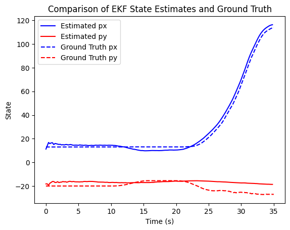
These deviations become more pronounced as the errors in observations and dynamics increase, especially towards the end of the time axis, where the accumulation of errors becomes too large for the EKF to correct.

This can be attributed to two possible reasons:

1. Our initial assumption that the sensor noise is Gaussian may be incorrect. If the noise is skewed in a non-Gaussian manner, it can cause errors to accumulate over time.

2. There might be unaccounted-for errors in the dynamics, and these errors may be non-Gaussian.

Conclusion

EKF relies heavily on matrix operations and linear algebra, which significantly reduces computation. However, it assumes Gaussian noise and the ability to linearize the system being estimated. This makes it suitable for many applications but inadequate for more complex, non-linear environments. When more computational power is available, other state estimation techniques, such as particle filters, offer a superior alternative. They can handle non-linearities and arbitrary noise distributions more effectively, although they require more complex mathematics and significantly higher computational resources. Despite the increased complexity, particle filters provide robust performance in a wider range of scenarios, making them a more versatile choice for challenging applications.

Here is the github repo for the problem statement and solution code.